Application of machine learning in rheumatic disease research

Article information

Korean J Intern Med. 2019;34(4):708-722

Publication date (electronic) : 2019 July 1

doi : https://doi.org/10.3904/kjim.2018.349

¹Division of Rheumatology, Department of Internal Medicine, College of Medicine, The Catholic University of Korea, Seoul, Korea

²Department of Computer Science, University of California, Davis, CA, USA

³Genome Center, University of California, Davis, CA, USA

Correspondence to Ki-Jo Kim, M.D. Division of Rheumatology, Department of Internal Medicine, College of Medicine, St. Vincent's Hospital, The Catholic University of Korea, 93 Jungbu-daero, Paldal-gu, Suwon 16247, Korea Tel: +82-31-249-8805 Fax: +82-31-253-8898 E-mail: md21c@catholic.ac.kr

Received 2018 September 23; Accepted 2018 November 18.

Abstract

Over the past decade, there has been a paradigm shift in how clinical data are collected, processed and utilized. Machine learning and artificial intelligence, fueled by breakthroughs in high-performance computing, data availability and algorithmic innovations, are paving the way to effective analyses of large, multi-dimensional collections of patient histories, laboratory results, treatments, and outcomes. In the new era of machine learning and predictive analytics, the impact on clinical decision-making in all clinical areas, including rheumatology, will be unprecedented. Here we provide a critical review of the machine-learning methods currently used in the analysis of clinical data, the advantages and limitations of these methods, and how they can be leveraged within the field of rheumatology.

Keywords: Rheumatology; Machine learning; Prediction

INTRODUCTION

Machine learning (ML) is a field of computer science that aims to create predictive models from data. It makes use of algorithms, methods and processes to uncover latent associations within the data and to create descriptive, predictive or prescriptive tools that exploit those associations [1]. It is often related to data mining [2], pattern recognition [3], artificial intelligence (AI) [4], and deep learning (DL) [5]. Although there are no clear definitions or boundaries among these areas and they often overlap, it is generally agreed that DL is a more recent sub-field of ML that uses computationally intensive algorithms and big data [6] to capture complex relationships within the data. Using multi-layered artificial neural networks, DL has dramatically improved the state-of-the-art in a variety of applications, including speech and visual object recognition, machine translation, natural language processing, and text automation [5,7]. Similarly, AI is broader than ML in that it uses the latter as a prediction engine feeding decision support and recommendation systems that are more than the sum of their parts. AI has been around for more than 70 years, born out of our appreciation and admiration of the power and inner workings of human intelligence [8]. Moreover, ML and AI are already part of our everyday lives, as they underlie our web searches [9], e-mail anti-spam filters [10], hotel and airline bookings [11], language translators [12], targeted advertising [13], and many other services [14]. Lately, ML and AI have captured the world's imagination in applications involving various complex games, with one of the most celebrated cases being the GO match held in 2016 between Sedol Lee, one of the top GO players in the world, and the computer program AlphaGo [5]. Fig. 1 provides a grouping of the different fields related to ML and AI.

Figure 1.

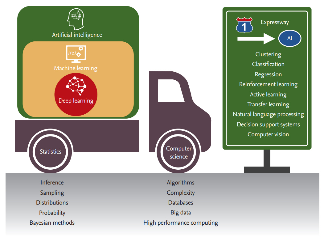
An overview of fields related to learning from data. AI, artificial intelligence.

The concept of ML dates to the 1940s but its development since the 1990s has been rapidly accelerated by the confluence of four key factors: the digitalization and storage of a massive amount of high-dimensional data at low cost; the development of general and graphic processors with high computational power; breakthroughs in ML algorithms that have significantly improved performance and minimized errors; and the free availability of open-source tools, codes, and models. In a clinical setting, ML and AI tools can help physicians ton understand a disease better and more accurately evaluate patients’ status based on high-throughput molecular and imaging techniques, which at the same time reveal the complexity and heterogeneity of the disease [15-17]. Nonetheless, equal to the promise of ML/AI are the potential dangers that may arise if too much trust is placed in automated diagnosis and decision tools. As a cautionary tale, the concordance between IBM’s Watson for Oncology [18] and an expert board of oncologists was highly variable, with a range of 17.8% to 97.9% depending on the tumor type, stage, hospital, and country [19]. Moreover, in recent news, the tool reportedly recommended unsafe cancer treatment plans [20]. Therefore, a thorough understanding and judicious approaches to ML are required to ensure its reasonable use in research and clinical practice. This is especially apparent given the complex nature of medicine, which involves the interactive combination of clinical and biological features in disease manifestation and diagnosis; a continuous inflow of new medical tools and drugs; socio-economic factors, such as the permission to treat that must be obtained from insurance companies; drug regulation and release by the regulatory agencies of the various countries; and ethical issues dealing with the use of electronic medical records (EMRs).

Rheumatic diseases, including rheumatoid arthritis (RA), systemic lupus erythematosus, Sjögren’s syndrome, systemic sclerosis, idiopathic inflammatory myositis, and the systemic vasculitides, are chronic autoimmune inflammatory disorders with multi-organ involvement. Complex interactions between a multitude of environmental and genetic factors affect disease development and progression [21,22]. In view of their heterogeneity, most rheumatic diseases are not defined as a single entity but as a single group according to established classification criteria [21,22]. Previous risk-prediction models for disease development and outcome based on population-wide databases work well on average, but in terms of precision medicine many of the diagnostic and management needs of patients with rheumatic diseases are still unmet [23,24]. In this setting, ML can suggest effective solutions for the unsettled issues arising from complex and heterogeneous diseases such as rheumatic diseases [16]. ML applications in multi-omics datasets were examined in detail in a series of recent reviews [7,25-29], and the superb performance of DL in image analysis has been the focus of recent papers [30-33]. Here we review the core principles and processes of ML that are applicable to clinical medicine as well as the current use of ML in research on rheumatic diseases. Our aim is to help clinicians and rheumatologists to understand better the basics of ML and its relevant research applications.

THE BASICS OF MACHINE LEARNING

Differences from traditional statistical models

There are substantial differences between ML and traditional statistics. First, ML concentrates on the task of “prediction,” by using general-purpose learning algorithms to find patterns in often rich and unwieldy data. By contrast, statistical methods have a long-standing focus on inference, which is achieved through the creation and fitting of a project-specific probability model [34]. Second, most ML techniques are hypothesis-free, as their aim is to reconstruct associations within the data, whereas traditional statistics usually rely on specific assumptions and hypotheses, often those stemming from the model that has generated the data [35]. Third, the toolsets used to evaluate the generalization errors of an ML model (receiver-operating characteristic curves, cross-validation, among others) are generally different from those of traditional statistical techniques, which mostly rely on a calculation of the p value to reject a null hypothesis [34,36,37]. Fourth, traditional statistical modeling is generally fitted to produce the simplest, most parsimonious model and yields a result that is easy to understand and interpret. However, clinical and biological factors are usually not independent of each other and their associations may be non-linear. ML approaches, however, consider all possible interactions between variables according to multi-dimensional non-linear patterns, irrespective of the degree of complexity, while aggressively seeking to capture as many informative and interesting features as possible. Nonetheless, by the same token, this can produce a complicated and sophisticated model that is not easy to understand or interpret. Fifth, it is often the case that the results of clinical studies are not consistent across studies, due to differences in the characteristics of the study population, the sample size or the measured variables (number, scale, and method). This is partly because traditional models seek a goodness of fit in a set of study samples. By contrast, the fundamental goal of ML is to generalize beyond the examples in the training set. Generalization is feasible because the models derive from a much larger dataset, are then validated in an independent dataset and further tuned to obtain the best performance [38,39].

Types of machine learning

There are many types of ML algorithms, as shown in Fig. 2. One of the most widely used categorizations separates them into three classes: supervised, unsupervised, and reinforcement learning.

Figure 2.

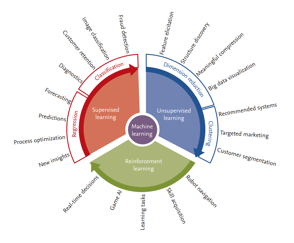
Overview of categorical types and different machine-learning algorithms. AI, artificial intelligence.

Supervised learning

Supervised learning searches for the relationship between a set of features (input variables) and one or more known outcomes (output classes or labels) and then derives a function that predicts the output value for a set of unlabeled input values based on an acceptable degree of fidelity [17,36,37]. For supervised learning to work, the training data should have the correct input-output pairs, which should be labeled by experts. Supervised learning includes both classification, where the task is to predict the group or class to which a new sample should be assigned (hence the output is a discrete variable), and regression, where the value of a continuous variable for a new sample must be estimated. For example, to determine whether a set of clinical features can predict the treatment response in patients with RA treated with a specific therapy, researchers can apply a supervised learning algorithm to a dataset in which each patient record contains the set of clinical features of interest and a label specifying the degree of disease responsiveness (e.g., “good,” “moderate,” “no” response, in conformity with the EULAR response criteria) [40]. Supervised learning algorithms include logistic and linear regression, naïve Bayesian classifiers, decision trees and random forests, support vector machines (SVMs), k-nearest neighbors, and neural networks [17,36,37].

Unsupervised learning

Unsupervised learning is a sub-field of ML that attempts to identify the structure in the data without the need for a training set, classes, or labels [17,36,37]. In the medical field, an example would be to identify hidden subsets of patients with similar clinical or molecular characteristics as described in the data. For example, patients with diffuse-type systemic sclerosis can be further categorized as having inflammatory, fibroproliferative, or normal-like disease based on their skin’s molecular signature [41,42]. The significance of this additional grouping can be further evaluated by determining correlations with clinical features and performance in subsequent supervised learning tasks. Unsupervised learning algorithms include clustering methods such as hierarchical or k-means clustering, principal component analysis, t-distributed stochastic neighbor embedding (t-SNE), non-negative matrix factorization, and latent class analysis [17,36,37,43].

Reinforcement learning

Reinforcement learning is an area of ML that is based on behavioral psychology, namely, how software agents take actions in a particular environment to maximize the cumulative reward [39]. The best example is game theory and the above-mentioned AlphaGo, which places a stone at a specific position on the board at a certain point in the game to maximize the winning rate [44]. A similar method was also used to select the best initial time for second-line therapy in patients with non-small cell lung cancer [45]. However, although it has great potential, reinforcement learning is not often applied to clinical settings, as it needs rigorously defined clinical states, observations (vitals, lab results, among others), and actions (treatment) and rewards, which are quite difficult to define and are sometimes unknown.

Transfer learning

Transfer learning is the improvement of the learning of a new task through the transfer of knowledge from a related task that has already been learned [46]. The assumption is that a model pre-trained in a dataset that has some similarities with the final dataset, i.e., the one that will ultimately be used for training, will perform better and be trained faster than if the model is exposed only to the latter. The two conditions under which this assumption holds true are: (1) the final dataset is much smaller than what is dictated by both the task at hand and the complexity of the model and (2) the pre-training dataset and the final dataset have some commonalities that are informative for that task. For example, assume that a model is to be trained to recognize black swans in images but only a few dozen images of swans of any kind are available; hence, the dataset is sufficient to train only the simplest of neural networks. In an alternative approach, large datasets comprising hundreds of thousands of images of birds in general can be substituted to pre-train the classifier to recognize birds. This pre-trained “bird” classifier can then be taught, using the key informative features of a bird (feathers, wings, beak, etc.), to recognize black swans from other items, including other birds. In a more relevant study for clinicians, Lakhani and Sundaram [47] adopted two famous deep convolutional neural network (DCNN) models for image classification, AlexNet [48] and GoogLeNet [49], pretrained on ImageNet [50], to differentiate pulmonary tuberculosis from the normal condition on a simple chest radiograph. DL with a DCNN accurately classified tuberculosis with an area under the curve (AUC) of 0.99.

SALIENT POINTS TO CONSIDER WHEN RUNNING MACHINE LEARNING

Medical or healthcare data can be presented in a table consisting of two components: rows of samples (observations or instances) and columns of features (variables or attributes). A schematic diagram of a supervised ML process is provided in Fig. 3. In data science, a programmed machine or model type is called a “learner.” In the following we discuss several points that should be kept in mind when ML is used.

Figure 3.

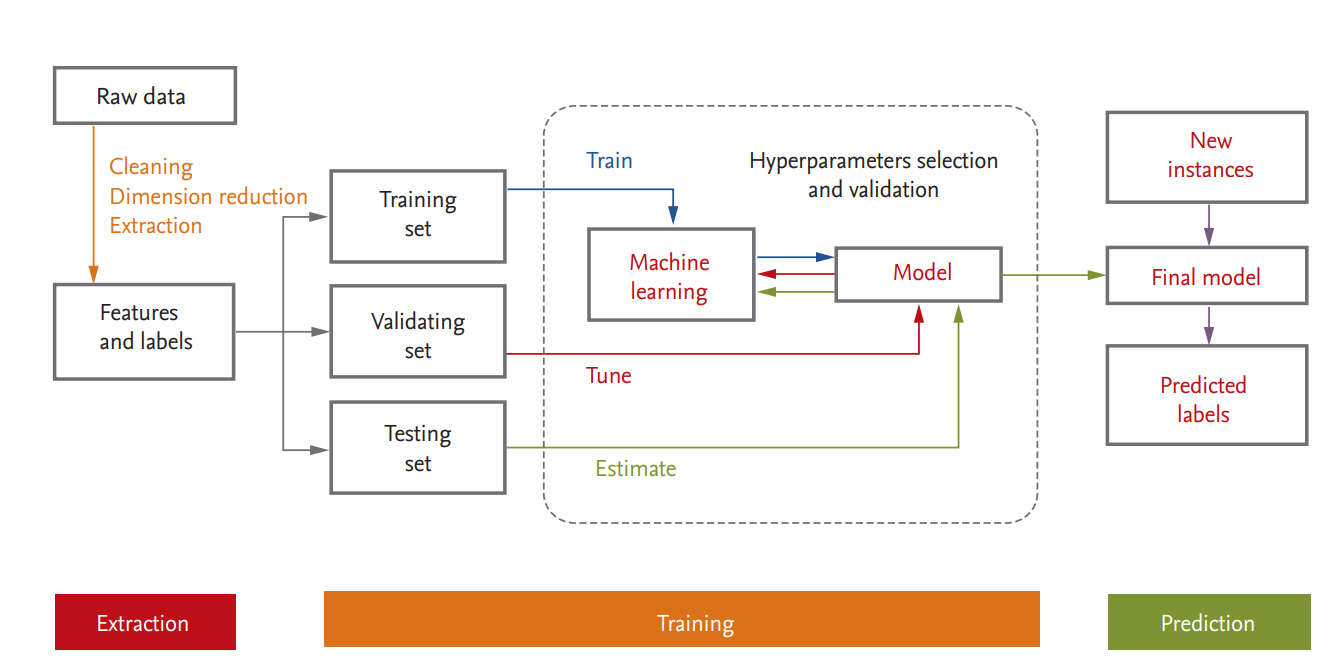
Workflow to develop a supervised machine-learning-based predictive model.

Data quantity, quality, and their control

In ML, the data are of high dimensionality and the sample size is large, so-called Big Data. An exploration of each subgroup of the data can reveal hidden structures by extracting important common features across many subgroups even when there are large individual variations. This is not feasible when the sample size is small because outliers may be mistakenly identified [51]. However, Big Data, a term applicable to EMRs, are inevitably characterized by certain weaknesses [51-53]. High dimensionality brings noise accumulation, spurious correlations, and incidental endogeneity [51]. In addition, because the massive samples in Big Data are typically aggregated from multiple sources at different times using different technologies, issues of heterogeneity, experimental variation, and statistical bias arise. Medical data are no exception, as there are clear differences between the formats used in EMRs, laboratory instruments, scales, assay reagents, and laboratory data notation methods. Furthermore, clinical and laboratory elements are often recorded incompletely or according to the preference of the particular doctor and therefore differently. In fact, the accuracy, completeness and comparability of EMR data were shown to vary from element to element by 10% to 90% [54]. The same disease code may be differently defined depending on the updated criteria, and coding errors inevitably occur because for the most part humans perform the recording. According to the Korean National Health Insurance claims database, true RA made up 91.4% of the total RA disease codes based on the RA identification algorithm [55]. Hence, to handle these challenges, aggressive quality control is needed [56], including data cleansing and refining techniques, such as error correction, removal of outliers, missing data interpolation, normalization, standardization, and de-batching. However, these processes rely on expert human judgment. Since even complex and sophisticated algorithms will not produce good results if the quality of the input data is poor, refinement of input data to improve their quality will provide better results even if the algorithm is less than optimal [37,57]. As has often been noted: “garbage in, garbage out” [58].

Data preprocessing

Raw data are usually not in a structure that is convenient for researchers to work with and not organized enough to be ready for ML. Data preprocessing refers to any transformation of the data before a learning algorithm is applied. It includes example finding and resolving inconsistencies; imputation of missing values; identifying, removing, or replacing outliers; discretizing numerical data or generating numerical dummy variables for categorical data; dimensionality reduction; feature extraction/selection; and feature scaling (normalization, standardization or Box-Cox transformation) [59]. Of these, feature scaling through standardization (or Z-score normalization) is an important preprocessing step for many ML algorithms. Predictor variables with ranges of different orders of magnitude can exert a disproportionate influence on the results. In other words, in the context of an algorithm, predictor variables with a greater range of scale may dominate. The scaling of feature values implicitly ensures equal weights of all features in their representation and should be the applied preprocessing approach in ML algorithms such as linear regression, SVM, and k-nearest neighbors [37].

Training, validation, and test datasets

For ML, the data are usually split into training, validation, and test datasets. The training dataset is the data sample used to fit the model. The validation dataset is the data sample used to provide an unbiased evaluation of a model fit on the training dataset while tuning model hyperparameters; it is regarded as a part of the training set. The test dataset is the data sample used to provide an unbiased evaluation of the fit that the final model achieved with the training dataset [36,37,60]. If the categorical variables are unbalanced, stratified sampling is favored. When a large amount of data is available, each set of samples can be set aside. However, if the number of samples is insufficient, removing data reduces the amount available for training. This can be mitigated by the use of resampling methods such as cross-validation and bootstrapping [60,61]. In general, a repeated 10-fold cross validation is recommended because of the low bias and variance properties of the performance estimate and the relatively low computational cost [37].

Bias-variance trade-off and overfitting

ML methods are often hindered by bias-variance trade-offs when a high-dimensional dataset with an inadequate number of samples is to be fitted [36,37,61]. Bias is the training error of the model; that is, the difference between the prediction value and the actual value. Models with a high bias tend to underfit, by applying a simpler model to describe a dataset of higher complexity. For example, if the goal is to capture the half-life relationship of protein degradation, a known non-linear process with exponential decay, the use of a linear model will not result in accurate prediction of protein levels at any time point, no matter how many training samples make up the dataset. By contrast, variance expresses the sensitivity of the model to small perturbations in the input. A model of high variance will provide substantially different answers (output values) for small changes in the input, because of overfitting of its parameters to the training dataset at hand [61]. This prevents generalizations (and thus the ability of the model to perform well) to other datasets never seen by the model, i.e., those it has not been trained on. In general, variance increases and bias decreases with increasing model complexity [36,62].

Many ML algorithms are susceptible to overfitting because they have a strong propensity to fit the model to the dataset and minimize the loss function as much as possible. Because the goal of ML is to make the model generalizable from learning the training data, and not to obtain the best model well-fitted for the training data, proper measures should be taken depending on the type of algorithm. The most popular solutions for overfitting are training with more data of high-quality and the least amount of noise, cross-validation, early stopping, pruning (remove features), regularization, and ensembling [36,37,61,63]. The appropriate combination should be selected depending on the purpose of the study, the characteristics and size of the dataset, and the learner type.

Feature engineering and selection

Since features describe the sample’s characteristics, more features imply a better understanding of the sample. However, in predictive modeling, too many features can impede learning because some may be irrelevant to the target of interest, less important than others or redundant in the context of other features. A “curse of dimensionality” occurs when the dimensionality of the data increases and the sparsity of the data increases [61]. It is statistically advantageous to estimate fewer parameters. In addition, researchers usually want to know the key informative features obtained with a simple model rather than work with a complex model that uses a large number of features to predict the outcome. In truth, processes that make the refined data amenable to learning, such as data cleaning, preprocessing, feature engineering and selection, are more essential than running a learner. However, this is a daunting task because it is manually tailored by domain experts in a time-consuming process [61]. Feature engineering is the process of transforming raw data such that the revised features better represent the problem that is of interest to the predictive model, resulting in improved model performance on new data. An example is to transform the counts of tender and/or swollen joints and the erythrocyte sedimentation rate (ESR) into a single formulated feature, Disease Activity Score (DAS28)-ESR, which better assesses disease activity in patients with RA. Feature selection is the process of selecting a subset of relevant features while pruning less-relevant features for use in model construction. There are three methods in feature selection algorithms: filter methods, wrapper methods, and embedded methods [37,64,65]. Filter methods involve the assignment of a score to each feature using a statistical measure followed by selection of high-ranked features based on the score. Filtering uses a preprocessing step and includes correlation coefficient scores, the pseudo-R² statistic and information gain. Wrapper methods evaluate multiple models using procedures that add and/or remove predictors to find the optimal combination that maximizes model performance. An example is the recursive feature elimination algorithm. Embedded methods perform variable selection in the process of training and are usually specific to certain learning machines. The most common type of embedded feature-selection method is the regularization method found in LASSO, Elastic Net, and Ridge regression. The features selected from the methods do not necessarily have a causal relationship with the target label, but simply provide critical information for use in predictive model construction.

Limitations of machine learning

ML has become ubiquitous and indispensable for solving complex problems in most sciences [16]. It can present novel findings or reveal previously hidden but important features that have been missed or overlooked in conventional studies using traditional statistics. However, those features might also be irrelevant, nonsensical, counterposed to the framework of current medical knowledge, or even cause confusion. This is because the results returned by ML are based solely on the input data. ML does not call the input data into question or explain why the results were obtained or their underlying mechanism. In the event of unexpected results, the data should be re-investigated to determine whether human or technical errors have created biases, followed by careful interpretation and validation in the context of the disease.

ML models are fairly dependent on the data they are trained on or are called upon to analyze, and no model, regardless of its sophistication, can create a useful analysis from low-quality data [61,66]. As data are a product made in the past and represent existing knowledge, ML models are valid within the same framework of that knowledge and their performance will degrade if they are not regularly updated using new, emerging data. In the case of a supervised classifier, a common problem is that the classes that make up the target label are not represented equally. An imbalanced distribution of class sizes across samples favors learning weighted to the larger class size such that the trained model then preferably assigns a major class label to new instances thereof while ignoring or misclassifying minority samples, which, although they rarely occur, might be very important. Several methods have been devised to handle the imbalanced class issue [67,68].

Because the optimal algorithm, i.e., the one that best fits the data of interest, cannot be known beforehand, a reasonable strategy is to sequentially test simple and widely known learners before moving on to those that are more sophisticated and distinct. In some ML learners, hyperparameters should be tuned by exhaustively searching through a manually specified subset of the hyperparameter space of a learning algorithm [69].

Randomness is an inherit characteristic of ML applications [70], appearing in data collections, observation orders, weight assignments, and resampling, among others. To create stable, robust models with reproducible results, detailed information on the type and version of the computational tools, learners’ parameters, hyperparameters and random seed number used should always be reported [71].

ILLUSTRATIVE EXAMPLES OF MACHINE LEARNING

Several representative clinical studies in which ML methods were used in the area of internal medicine are summarized in Table 1 [72-86]. In the study of rheumatic diseases, ML has been employed only recently, but two of those studies are particularly noteworthy. In the first, Orange et al. [87] reported the identification of three distinct synovial subtypes based on the synovial gene signatures of patients with RA. These labels were used to design a histologic scoring algorithm in which the histologic scores correlated with clinical parameters such as ESR, C-reactive protein (CRP) level, and autoantibody titer [87]. The authors selected 14 histologic features from 129 synovial samples (123 RA and six osteoarthritis [OA] patients) and the 500 most variably expressed genes in 45 synovial samples (from 39 RA and six OA patients). Gene-expression-driven subgrouping was explored by k-means clustering, in which n objects are partitioned into k clusters, with each object belonging to the cluster with the nearest mean [88]. Clustering was most robust at 3 and this subgrouping was validated by principal component analysis, but not in an independent dataset. Three subgroups comprising high-inflammatory, low-inflammatory, and mixed subtypes, were designated based on their gene patterns and enriched ontology. The aim of the study was to determine the synchrony between synovial histologic features and genomic subtype, thereby yielding a convenient histology-based approach to characterization of synovial tissue. To this end, a leave-one-out cross-validation SVM classifier was implemented. The aim of an SVM is to find a decision hyperplane that separates data points of different classes with a maximal margin (i.e., the maximal distance to the nearest training data points) [89]. The model’s performance in separating both the high and the low inflammatory subtypes from the other subtypes was relatively good (AUCs of 0.88 and 0.71, respectively). It should be noted that histologic subtypes are closely associated with clinical features, as significant increases in ESR, CRP levels, rheumatoid factor titer, and anti-cyclic citrullinated protein (CCP) titer in patients with high inflammatory scores were detected. However, this model might succumb to overfitting because SVM is vulnerable to overfitting [89,90], the sample size was too small (only 45 samples) and the model was not validated using an independent dataset. Moreover, the data samples were a mixture of RA and OA samples and there were no normal controls. SVM is an unsupervised ML with an efficient performance achieved using the kernel trick and the tuning of hyperparameters. A better approach would be to specify the details of the model (kernel type, parameters, and hyperparameters) during method selection, to guarantee the reliability and reproducibility of the model.

Table 1.

Representative clinical studies using machine learning methods in internal medicine

In the second, Lezcano-Valverde et al. [91] developed and validated a random survival forest (RSF) prediction model of mortality in RA patients based on demographic and clinically related variables. RSF, an extension of random forest for time-to-event data, is a non-parametric method that generates multiple decision trees using a bagging method [92,93]. Bagging, an abbreviation for bootstrap aggregation, is a simple and powerful ensemble method that fits multiple predictive models on random subsets of the original dataset and aggregates their individual predictions by either voting or averaging [94]. It is commonly used to reduce variance and avoid overfitting. RSF is an attractive alternative to the Cox proportional hazards model when the proportional hazards assumption is violated [93,95]. Lezcano-Valverde et al. [91] used two independent cohorts as the training and validation datasets: the RA cohort from the Hospital Clínico San Carlos (HCSC-RAC), consisting of 1,461 patients, and the 280 RA patients from the Hospital Universitario de La Princesa Early Arthritis Register Longitudinal (PEARL) study. Each model was run 100 times using 1,000 trees per run. The prediction error was 0.187 in the training cohort and 0.233 in the validation cohort. Important variables with a higher predictive capacity were age at diagnosis, median ESR and number of hospital admissions. These variables were consistent with those obtained in a previous result using a Cox proportional hazards model [96]. The strengths of the approach described in that study were external validation using an independent RA cohort and the absence of a restrictive assumption, which traditional Cox proportional hazards model rely on. RSF has also been used to analyze the mortality risk in patients with systemic lupus erythematosus [97] and in those with juvenile idiopathic inflammatory myopathies [98].

CONCLUSIONS

ML algorithms can accommodate diverse configurations of data, specify context weighting, and identify informative patterns that enable subgrouping or predictive modeling from every interaction of variables available for the assessment of diagnostic and prognostic elements. Extensive, in-depth applications of ML in biomedical science are increasing in number, and interesting results in the area of precision medicine have been obtained. However, several challenges must still be overcome. First, ML works only if the training data are representative of the problem to be solved, include informative features and are of sufficient quantity to train the model at hand. This can be difficult to achieve for both technical and real-world reasons. Second, privacy is a major concern in the collection of sensitive clinical data, which might limit the aggregation of all necessary information. Moreover, some data are expensive to acquire, reported in different formats and obtained using different methods and technologies. Third, because text-based medical records can be incoherent, distracted, and contain technical errors [52,53], expert human judgement is needed to review the data, detect any errors or problems and determine the clinical significance of any findings [35,99]. Finally, a consensus should be reached on how to integrate and coordinate ML results with previously established guidelines or recommendations that were based on traditional statistics.

ML and AI will change the clinical landscape as we know it. From clinical decision support tools and personalized recommendation systems to the discovery of novel drugs and treatments, AI is poised to propel our world to unprecedented levels of automation, personalized service and accelerated R&D cycles. Close collaboration and interdisciplinary teamwork between clinicians, biomedical informatics scientists, ML experts, and administrative stakeholders are a prerequisite to the achievement of satisfactory solutions amenable to a variety of clinical applications.

Notes

No potential conflict of interest relevant to this article was reported.

References

1. Samuel AL. Some studies in machine learning using the game of checkers. IBM J Res Dev 1959;3:210–229.

2. Witten IH, Frank E, Hall MA, Pal CJ. Data Mining: Practical Machine Learning Tools and Techniques 4th edth ed. Cambridge (MA): Elsevier Science; 2016.

3. Nasrabadi NM. Pattern recognition and machine learning. J Electron Imaging 2007;16:049901.

4. Michalski RS, Carbonell JG, Mitchell TM. Machine Learning: An Artificial Intelligence Approach Berlin (DE): Springer Berlin Heidelberg; 2013.

5. LeCun Y, Bengio Y, Hinton G. Deep learning. Nature 2015;521:436–444.

6. Najafabadi MM, Villanustre F, Khoshgoftaar TM, Seliya N, Wald R, Muharemagic E. Deep learning applications and challenges in big data analytics. J Big Data 2015;2:1.

7. Ching T, Himmelstein DS, Beaulieu-Jones BK, et al. Opportunities and obstacles for deep learning in biology and medicine. J R Soc Interface 2018;15:20170387.

8. Hamet P, Tremblay J. Artificial intelligence in medicine. Metabolism 2017;69S:S36–S40.

9. Boyan J, Freitag D, Joachims T. A machine learning architecture for optimizing web search engines. AAAI Workshop on Internet Based Information Systems 1996 May 10. Portland: OR.

10. Guzella TS, Caminhas WM. A review of machine learning approaches to spam filtering. Expert Syst Appl 2009;36:10206–10222.

11. Etzioni O, Tuchinda R, Knoblock CA, Yates A. To buy or not to buy: mining airfare data to minimize ticket purchase price. In : Proceedings of the ninth ACM SIGKDD international conference on Knowledge discovery and data mining; 2003 Aug 24-27; Washington, DC. New York (NY). ACM. 2003. 119–128.

12. Bahdanau D, Cho K, Bengio Y. Neural machine translation by jointly learning to align and translate. In : International Conference on Learning Representations; 2015. 2015 May 7-9; San Diego, CA.

13. Perlich C, Dalessandro B, Raeder T, Stitelman O, Provost F. Machine learning for targeted display advertising: transfer learning in action. Mach Learn 2014;95:103–127.

14. Rabunal JR, Dorrado J. Artificial Neural Networks in Real-Life Applications Hershey (PA): Idea Group Pub; 2006.

15. Krittanawong C, Zhang H, Wang Z, Aydar M, Kitai T. Artificial intelligence in precision cardiovascular medicine. J Am Coll Cardiol 2017;69:2657–2664.

16. Obermeyer Z, Emanuel EJ. Predicting the future: big data, machine learning, and clinical medicine. N Engl J Med 2016;375:1216–1219.

17. Sanchez-Pinto LN, Luo Y, Churpek MM. Big data and data science in critical care. Chest 2018;154:1239–1248.

18. Curioni-Fontecedro A. A new era of oncology through artificial intelligence. ESMO Open 2017;2e000198.

19. Choi YS. Concepts, characteristics, and clinical validation of IBM Watson for oncology. Hanyang Med Rev 2017;37:49–60.

20. Ross C, Swetlitz I. IBM’s Watson supercomputer recommended ‘unsafe and incorrect’ cancer treatments, internal documents show [Internet]. Boston (MA): STAT; c2018. [cited 2018 Nov 14]. Available from: https://www.statnews.com/2018/07/25/ibm-watson-recommended-unsafe-incorrect-treatments/.

21. Goldblatt F, O'Neill SG. Clinical aspects of autoimmune rheumatic diseases. Lancet 2013;382:797–808.

22. Smolen JS, Aletaha D, McInnes IB. Rheumatoid arthritis. Lancet 2016;388:2023–2038.

23. Giacomelli R, Afeltra A, Alunno A, et al. International consensus: what else can we do to improve diagnosis and therapeutic strategies in patients affected by autoimmune rheumatic diseases (rheumatoid arthritis, spondyloarthritides, systemic sclerosis, systemic lupus erythematosus, antiphospholipid syndrome and Sjogren's syndrome)? The unmet needs and the clinical grey zone in autoimmune disease management. Autoimmun Rev 2017;16:911–924.

24. Winthrop KL, Strand V, van der Heijde D, et al. The unmet need in rheumatology: reports from the targeted therapies meeting 2017. Clin Immunol 2018;186:87–93.

25. Larranaga P, Calvo B, Santana R, et al. Machine learning in bioinformatics. Brief Bioinform 2006;7:86–112.

26. Libbrecht MW, Noble WS. Machine learning applications in genetics and genomics. Nat Rev Genet 2015;16:321–332.

27. Noell G, Faner R, Agusti A. From systems biology to P4 medicine: applications in respiratory medicine. Eur Respir Rev 2018;27:170110.

28. Kim M, Tagkopoulos I. Data integration and predictive modeling methods for multi-omics datasets. Mol Omics 2018;14:8–25.

29. Wainberg M, Merico D, Delong A, Frey BJ. Deep learning in biomedicine. Nat Biotechnol 2018;36:829–838.

30. Chartrand G, Cheng PM, Vorontsov E, et al. Deep learning: a primer for radiologists. Radiographics 2017;37:2113–2131.

31. Lee JG, Jun S, Cho YW, et al. Deep learning in medical imaging: general overview. Korean J Radiol 2017;18:570–584.

32. Parmar C, Barry JD, Hosny A, Quackenbush J, Aerts HJWL. Data analysis strategies in medical imaging. Clin Cancer Res 2018;24:3492–3499.

33. Shen D, Wu G, Suk HI. Deep learning in medical image analysis. Annu Rev Biomed Eng 2017;19:221–248.

34. Bzdok D, Altman N, Krzywinski M. Statistics versus machine learning. Nat Methods 2018;15:233–234.

35. Waljee AK, Higgins PD. Machine learning in medicine: a primer for physicians. Am J Gastroenterol 2010;105:1224–1226.

36. James G, Witten D, Hastie T, Tibshirani R. An Introduction to Statistical Learning: With Applications in R New York (NY): Springer New York; 2013.

37. Kuhn M, Johnson K. Applied Predictive Modeling New York (NY): Springer New York; 2013.

38. Handelman GS, Kok HK, Chandra RV, Razavi AH, Lee MJ, Asadi H. eDoctor: machine learning and the future of medicine. J Intern Med 2018;284:603–619.

39. Shameer K, Johnson KW, Glicksberg BS, Dudley JT, Sengupta PP. Machine learning in cardiovascular medicine: are we there yet? Heart 2018;104:1156–1164.

40. van Gestel AM, Prevoo ML, van 't Hof MA, van Rijswijk MH, van de Putte LB, van Riel PL. Development and validation of the European League Against Rheumatism response criteria for rheumatoid arthritis. Comparison with the preliminary American College of Rheumatology and the World Health Organization/International League Against Rheumatism Criteria. Arthritis Rheum 1996;39:34–40.

41. Milano A, Pendergrass SA, Sargent JL, et al. Molecular subsets in the gene expression signatures of scleroderma skin. PLoS One 2008;3e2696.

42. Pendergrass SA, Lemaire R, Francis IP, Mahoney JM, Lafyatis R, Whitfield ML. Intrinsic gene expression subsets of diffuse cutaneous systemic sclerosis are stable in serial skin biopsies. J Invest Dermatol 2012;132:1363–1373.

43. Magidson J, Vermunt J. Latent class models for clustering: A comparison with K-means. Can J Mark Res 2002;20:36–43.

44. Silver D, Huang A, Maddison CJ, et al. Mastering the game of Go with deep neural networks and tree search. Nature 2016;529:484–489.

45. Zhao Y, Zeng D, Socinski MA, Kosorok MR. Reinforcement learning strategies for clinical trials in nonsmall cell lung cancer. Biometrics 2011;67:1422–1433.

46. Torrey L, Shavlik J. Transfer learning. In : Olivas ES, ed. Handbook of Research on Machine Learning Applications and Trends: Algorithms, Methods, and Techniques Hershey, PA: IGI Global; 2010. p. 242–264.

47. Lakhani P, Sundaram B. Deep learning at chest radiography: automated classification of pulmonary tuberculosis by using convolutional neural networks. Radiology 2017;284:574–582.

48. Krizhevsky A, Sutskever I, Hinton GE. Imagenet classification with deep convolutional neural networks. In : Advances in neural information processing systems 25; 2012 Dec 3-6; Lake Tahoe, NV. Red Hook (NY). In : Curran Associates; 2012. 1097–1105.

49. He K, Zhang X, Ren S, Sun J. Delving deep into rectifiers: surpassing human-level performance on imagenet classification. In : Proceedings of the 2015 IEEE International Conference on Computer Vision; 2015 Dec 7-13; Santiago, Chile. Piscataway (NJ). In : IEEE; 2015. 1026–1034.

50. Deng J, Dong W, Socher R, Li LJ, Li K, Fei-Fei L. Imagenet: a large-scale hierarchical image database. In : 2009 IEEE Conference on Computer Vision and Pattern Recognition; 2009 Jun 20-25; Miami, FL. Piscataway (NJ). In : IEEE; 2009. 248–255.

51. Fan J, Han F, Liu H. Challenges of big data analysis. Natl Sci Rev 2014;1:293–314.

52. Alpert JS. The electronic medical record in 2016: advantages and disadvantages. Digit Med 2016;2:48–51.

53. Menachemi N, Collum TH. Benefits and drawbacks of electronic health record systems. Risk Manag Healthc Policy 2011;4:47–55.

54. Chan KS, Fowles JB, Weiner JP. Review: electronic health records and the reliability and validity of quality measures. A review of the literature. Med Care Res Rev 2010;67:503–527.

55. Cho SK, Sung YK, Choi CB, Kwon JM, Lee EK, Bae SC. Development of an algorithm for identifying rheumatoid arthritis in the Korean National Health Insurance claims database. Rheumatol Int 2013;33:2985–2992.

56. Redman TC. If your data is bad, your machine learning tools are useless [Internet]. Boston (MA): Harvard Business Publishing; c2018. [cited 2018 Nov 15]. Available from: https://hbr.org/2018/04/if-your-data-is-bad-your-machine-learning-tools-are-useless.

57. Cherkassky VS, Mulier FM. Learning from Data: Concepts, Theory, and Methods 2nd edth ed. Hoboken (NJ): Wiley; 2007.

58. Kilkenny MF, Robinson KM. Data quality: "Garbage in-garbage out". Health Inf Manag 2018;47:103–105.

59. Kotsiantis SB, Kanellopoulos D, Pintelas PE. Data preprocessing for supervised leaning. Int J Comput Electr Autom Control Inf Eng 2006;1:111–117.

60. Kohavi R. A study of cross-validation and bootstrap for accuracy estimation and model selection. In : Proceedings of the 14th international joint conference on Artificial intelligence volume 2; 1995 Aug 20-25; Montreal, QC. San Mateo (CA). In : Morgan Kaufmann Publishers Inc; 1995. 1137–1143.

61. Domingos P. A few useful things to know about machine learning. Commun ACM 2012;55:78–87.

62. Lever J, Krzywinski M, Altman N. Points of significance: model selection and overfitting. Nat Methods 2016;13:703–704.

63. Hawkins DM. The problem of overfitting. J Chem Inf Comput Sci 2004;44:1–12.

64. Guyon I, Elisseeff A. An introduction to variable and feature selection. J Mach Learn Res 2003;3:1157–1182.

65. Saeys Y, Inza I, Larranaga P. A review of feature selection techniques in bioinformatics. Bioinformatics 2007;23:2507–2517.

66. Banko M, Brill E. Scaling to very very large corpora for natural language disambiguation. In : Proceedings of the 39th Annual Meeting on Association for Computational Linguistics; 2001 Jul 6-11; Toulouse, France. San Francisco (CA). In : Morgan Kaufmann Publishers; 2001. 26–33.

67. Longadge R, Dongre S, Malik L. Class imbalance problem in data mining: review. Int J Comput Sci Netw 2013;2:83–87.

68. Saito T, Rehmsmeier M. The precision-recall plot is more informative than the ROC plot when evaluating binary classifiers on imbalanced datasets. PLoS One 2015;10e0118432.

69. Claesen M, De Moor B. Hyperparameter search in machine learning. Int J Comput Sci Netw 2015. 41–5. https://arxiv.org/abs/1502.02127.

70. Ben-David A. A lot of randomness is hiding in accuracy. Eng Appl Artif Intell 2007;20:875–885.

71. Piccolo SR, Frampton MB. Tools and techniques for computational reproducibility. Gigascience 2016;5:30.

72. Hsich E, Gorodeski EZ, Blackstone EH, Ishwaran H, Lauer MS. Identifying important risk factors for survival in patient with systolic heart failure using random survival forests. Circ Cardiovasc Qual Outcomes 2011;4:39–45.

73. Gorodeski EZ, Ishwaran H, Kogalur UB, et al. Use of hundreds of electrocardiographic biomarkers for prediction of mortality in postmenopausal women: the Women's Health Initiative. Circ Cardiovasc Qual Outcomes 2011;4:521–532.

74. Shah SJ, Katz DH, Selvaraj S, et al. Phenomapping for novel classification of heart failure with preserved ejection fraction. Circulation 2015;131:269–279.

75. Motwani M, Dey D, Berman DS, et al. Machine learning for prediction of all-cause mortality in patients with suspected coronary artery disease: a 5-year multicentre prospective registry analysis. Eur Heart J 2017;38:500–507.

76. Guan WJ, Jiang M, Gao YH, et al. Unsupervised learning technique identifies bronchiectasis phenotypes with distinct clinical characteristics. Int J Tuberc Lung Dis 2016;20:402–410.

77. Waljee AK, Lipson R, Wiitala WL, et al. Predicting hospitalization and outpatient corticosteroid use in inflammatory bowel disease patients using machine learning. Inflamm Bowel Dis 2017;24:45–53.

78. Koyner JL, Carey KA, Edelson DP, Churpek MM. The development of a machine learning inpatient acute kidney injury prediction model. Crit Care Med 2018;46:1070–1077.

79. Kleiman RS, LaRose ER, Badger JC, et al. Using machine learning algorithms to predict risk for development of calciphylaxis in patients with chronic kidney disease. AMIA Jt Summits Transl Sci Proc 2018;2017:139–146.

80. Allalou A, Nalla A, Prentice KJ, et al. A predictive metabolic signature for the transition from gestational diabetes mellitus to type 2 diabetes. Diabetes 2016;65:2529–2539.

81. Farran B, Channanath AM, Behbehani K, Thanaraj TA. Predictive models to assess risk of type 2 diabetes, hypertension and comorbidity: machine-learning algorithms and validation using national health data from Kuwait. A cohort study. BMJ Open 2013;3e002457.

82. Beck AH, Sangoi AR, Leung S, et al. Systematic analysis of breast cancer morphology uncovers stromal features associated with survival. Sci Transl Med 2011;3:108ra113.

83. Cheng WY, Ou Yang TH, Anastassiou D. Development of a prognostic model for breast cancer survival in an open challenge environment. Sci Transl Med 2013;5:181ra50.

84. Yu KH, Zhang C, Berry GJ, et al. Predicting non-small cell lung cancer prognosis by fully automated microscopic pathology image features. Nat Commun 2016;7:12474.

85. Shouval R, Labopin M, Bondi O, et al. Prediction of allogeneic hematopoietic stem-cell transplantation mortality 100 days after transplantation using a machine learning algorithm: a European group for blood and marrow transplantation acute leukemia working party retrospective data mining study. J Clin Oncol 2015;33:3144–3151.

86. Esteva A, Kuprel B, Novoa RA, et al. Dermatologist-level classification of skin cancer with deep neural networks. Nature 2017;542:115–118.

87. Orange DE, Agius P, DiCarlo EF, et al. Identification of three rheumatoid arthritis disease subtypes by machine learning integration of synovial histologic features and RNA sequencing data. Arthritis Rheumatol 2018;70:690–701.

88. Kanungo T, Mount DM, Netanyahu NS, Piatko CD, Silverman R, Wu AY. An efficient k-means clustering algorithm: analysis and implementation. IEEE Trans Pattern Anal Mach Intell 2002;24:881–892.

89. Noble WS. What is a support vector machine? Nat Biotechnol 2006;24:1565–1567.

90. Han H, Jiang X. Overcome support vector machine diagnosis overfitting. Cancer Inform 2014;13(Suppl 1):145–158.

91. Lezcano-Valverde JM, Salazar F, Leon L, et al. Development and validation of a multivariate predictive model for rheumatoid arthritis mortality using a machine learning approach. Sci Rep 2017;7:10189.

92. Ishwaran H, Kogalur UB, Blackstone EH, Lauer MS. Random survival forests. Ann Appl Stat 2008;2:841–860.

93. Ehrlinger J. ggRandomForests: exploring random forest survival [Internet]. ArXiv: 2016. [cited 2018 Nov 15]. Available from: https://arxiv.org/abs/1612.08974.

94. Altman N, Krzywinski M. Ensemble methods: bagging and random forests. Nat Methods 2017;14:933–934.

95. Nasejje JB, Mwambi H, Dheda K, Lesosky M. A comparison of the conditional inference survival forest model to random survival forests based on a simulation study as well as on two applications with time-to-event data. BMC Med Res Methodol 2017;17:115.

96. Abasolo L, Ivorra-Cortes J, Leon L, Jover JA, Fernandez-Gutierrez B, Rodriguez-Rodriguez L. Influence of demographic and clinical factors on the mortality rate of a rheumatoid arthritis cohort: a 20-year survival study. Semin Arthritis Rheum 2016;45:533–538.

97. Ward MM, Pajevic S, Dreyfuss J, Malley JD. Short-term prediction of mortality in patients with systemic lupus erythematosus: classification of outcomes using random forests. Arthritis Rheum 2006;55:74–80.

98. Huber AM, Mamyrova G, Lachenbruch PA, et al. Early illness features associated with mortality in the juvenile idiopathic inflammatory myopathies. Arthritis Care Res (Hoboken) 2014;66:732–740.

99. Data glitches are hazardous to your health. Sci Am 2013;309:10.

Article information Continued

This is an Open Access article distributed under the terms of the Creative Commons Attribution Non-Commercial License (http://creativecommons.org/licenses/by-nc/4.0/) which permits unrestricted noncommercial use, distribution, and reproduction in any medium, provided the original work is properly cited.

Area	Title	Machine learning category	Machine learning methods	Input data	Reference
Cardiology	Identifying important risk factors for survival in patient with systolic heart failure using random survival forests	Supervised	Random survival forest	39 Clinical variables	[72]
Cardiology		Supervised	Random survival forest	2,231 Adult patients with systolic heart failure	[72]
Cardiology	Use of hundreds of electrocardiographic biomarkers for prediction of mortality in postmenopausal women: the Women's Health Initiative	Supervised	Random survival forest	477 Electrocardiographic findings	[73]
Cardiology		Supervised	Random survival forest	33,144 Postmenopausal women	[73]
Cardiology	Phenomapping for novel classification of heart failure with preserved ejection fraction	Unsupervised	Agglomerative hierarchical clustering	67 Clinical and echocardiographic parameters	[74]
Cardiology		Unsupervised	Agglomerative hierarchical clustering	420 Patients with heart failure with preserved ejection fraction	[74]
Cardiology	Machine learning for prediction of all-cause mortality in patients with suspected coronary artery disease: a 5-year multicentre prospective registry analysis	Supervised	Logit-boost model	44 Coronary computed tomographic angiography variables and 25 clinical variables	[75]
Cardiology		Supervised	Logit-boost model	10,030 Patients with suspected coronary artery disease	[75]
Pulmonology	Unsupervised learning technique identifies bronchiectasis phenotypes with distinct clinical characteristics	Unsupervised	Hierarchical clustering	78 Selected features from clinical, radiographic, and functional parameters	[76]
Pulmonology		Unsupervised	Hierarchical clustering	148 Patients with bronchiectasis	[76]
Gastroenterology	Predicting hospitalization and outpatient corticosteroid use in inflammatory bowel disease patients using machine learning	Supervised	Random forest	Over 30 clinical and laboratory features	[77]
Gastroenterology		Supervised	Random forest	20,368 Patients with inflammatory bowel disease	[77]
Nephrology	The development of a machine learning inpatient acute kidney injury prediction model	Supervised	Gradient boosting machine	36 Clinical and laboratory features	[78]
Nephrology		Supervised	Gradient boosting machine	121,158 Admissions	[78]
Nephrology	Using machine learning algorithms to predict risk for development of calciphylaxis in patients with chronic kidney disease	Supervised	LASSO logistic regression	9,288 Clinical and laboratory features	[79]
Nephrology		Supervised	Random forest	401 Patients with chronic kidney disease	[79]
Endocrinology	A predictive metabolic signature for the transition from gestational diabetes mellitus to type 2 diabetes	Supervised	Decision tree (J48)	110 Blood metabolites	[80]
Endocrinology		Supervised	Naïve Bayes classifier	1,035 Women with gestational diabetes	[80]
Endocrinology	Predictive models to assess risk of type 2 diabetes, hypertension and comorbidity: machine-learning algorithms and validation using national health data from Kuwait. A cohort study	Supervised	Logistic regression	13,647,408 Variables in medical records	[81]
			k-Nearest neighbors	300,489 Hospital visitors
			Support vector machines
			Multifactor dimensionality reduction
Oncology	Systematic analysis of breast cancer morphology uncovers stromal features associated with survival	Supervised	LASSO logistic regression	6,642 Image features from H&E-stained histological images	[82]
Oncology		Supervised	LASSO logistic regression	Two independent sets of patients with breast cancer: NKI (248 patients) and VGH (328 patients)	[82]
Oncology	Development of a prognostic model for breast cancer survival in an open challenge environment	Supervised Unsupervised	Attractor metagenes analysis	Clinical, survival information and 12 molecular features	[83]
			Generalized boosted regression	1,981 Patients with breast cancer
			k-Nearest neighbors	1,981 Patients with breast cancer
Oncology	Predicting non-small cell lung cancer prognosis by fully automated microscopic pathology image features	Supervised	Naïve Bayes classifiers	9,879 Image features	[84]
			Support vector machines	2,186 H&E stained whole-slide histopathology images, which were obtained from 515 lung adenocarcinoma patients and 502 lung squamous cell carcinoma patients.
			Random forest
Hematology	Prediction of allogeneic hematopoietic stem- cell transplantation mortality 100 days after transplantation using a machine learning algorithm: a European group for blood and marrow transplantation acute leukemia working party retrospective data mining study	Supervised	Alternating decision tree	18 Clinical features	[85]
Hematology		Supervised	Alternating decision tree	28,236 Adult hematopoietic stem cell transplantation recipients who were affected by acute leukemia	[85]
Dermatology	Dermatologist-level classification of skin cancer with deep neural networks	Supervised	Deep convolutional neural network	129,450 Clinical images of skin lesions, which were labeled with 2,032 various skin disease	[86]